SPSS 스타일로 데이터 분석하기

R 2018. 12. 27. 19:00

유용한 패키지를 발견했다.

마케팅 분야나 사회조사에서 빈도표와 교차표(분할표)를 아주 많이 사용하고 있다. 얼마전에 강의했던 곳에서도 SPSS를 대체해서 R로 데이터분석을 하고 싶은데, 가장 많은 질문은 SPSS로 작성하는 빈도표나 교차표를 어떻게 R에서 작성하는 지를 많이 질문했다. 또한 변수가 가지는 값에 대한 설명의 설정도 질문했다.

이 질문에 대답이 될 수 있는 하나의 패키지이다.
바로 expss 이다.

아래의 사이트를 참고하면 많은 도움이 될 것 같다.
https://gdemin.github.io/expss/

앞으로 이 부분을 잘 학습해서,
마케팅 관련된 분야에서 근무하시는 사람들을 위한 책이나 강의를 해야겠다.

Introduction

expss package provides tabulation functions with support for ‘SPSS’-style labels, multiple / nested banners, weights, multiple-response variables and significance testing. There are facilities for nice output of tables in ‘knitr’, R notebooks, ‘Shiny’ and ‘Jupyter’ notebooks. Proper methods for labelled variables add value labels support to base R functions and to some functions from other packages. Additionally, the package offers useful functions for data processing in marketing research / social surveys - popular data transformation functions from ‘SPSS’ Statistics (‘RECODE’, ‘COUNT’, ‘COMPUTE’, ‘DO IF’, etc.) and ‘Excel’ (‘COUNTIF’, ‘VLOOKUP’, etc.). Package is intended to help people to move data processing from ‘Excel’/‘SPSS’ to R. See examples below. You can get help about any function by typing ?function_name in the R console.

Installation

expss is on CRAN, so for installation you can print in the console install.packages("expss").

Cross-tablulation examples

We will use for demonstartion well-known mtcars dataset. Let’s start with adding labels to the dataset. Then we can continue with tables creation.

library(expss)
data(mtcars)
mtcars = apply_labels(mtcars,
                      mpg = "Miles/(US) gallon",
                      cyl = "Number of cylinders",
                      disp = "Displacement (cu.in.)",
                      hp = "Gross horsepower",
                      drat = "Rear axle ratio",
                      wt = "Weight (1000 lbs)",
                      qsec = "1/4 mile time",
                      vs = "Engine",
                      vs = c("V-engine" = 0,
                             "Straight engine" = 1),
                      am = "Transmission",
                      am = c("Automatic" = 0,
                             "Manual"=1),
                      gear = "Number of forward gears",
                      carb = "Number of carburetors"
)

For quick cross-tabulation there are fre and cro family of function. For simplicity we demonstrate here only cro_cpct which caluclates column percent. Documentation for other functions, such as cro_cases for counts, cro_rpct for row percent, cro_tpctfor table percent and cro_fun for custom summary functions can be seen by typing ?cro and ?cro_fun in the console.

# 'cro' examples
# just simple crosstabulation, similar to base R 'table' function
cro(mtcars$am, mtcars$vs)

	Engine
	V-engine	Straight engine
Transmission
Automatic	12	7
Manual	6	7
#Total cases	18	14

# Table column % with multiple banners
cro_cpct(mtcars$cyl, list(total(), mtcars$am, mtcars$vs))

	#Total	Transmission		Engine
		Automatic	Manual	V-engine	Straight engine
Number of cylinders
4	34.4	15.8	61.5	5.6	71.4
6	21.9	21.1	23.1	16.7	28.6
8	43.8	63.2	15.4	77.8
#Total cases	32	19	13	18	14

# or, the same result with another notation
mtcars %>% calc_cro_cpct(cyl, list(total(), am, vs))

	#Total	Transmission		Engine
		Automatic	Manual	V-engine	Straight engine
Number of cylinders
4	34.4	15.8	61.5	5.6	71.4
6	21.9	21.1	23.1	16.7	28.6
8	43.8	63.2	15.4	77.8
#Total cases	32	19	13	18	14

# Table with nested banners (column %).          
mtcars %>% calc_cro_cpct(cyl, list(total(), am %nest% vs))

	#Total	Transmission
		Automatic		Manual
		Engine		Engine
		V-engine	Straight engine	V-engine	Straight engine
Number of cylinders
4	34.4		42.9	16.7	100
6	21.9		57.1	50.0
8	43.8	100		33.3
#Total cases	32	12	7	6	7

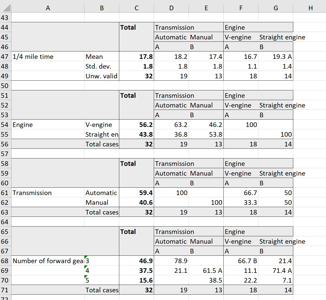
We have more sophisticated interface for table construction with magrittr piping. Table construction consists of at least of three functions chained with pipe operator: %>%. At first we need to specify variables for which statistics will be computed with tab_cells. Secondary, we calculate statistics with one of the tab_stat_* functions. And last, we finalize table creation with tab_pivot, e. g.: dataset %>% tab_cells(variable) %>% tab_stat_cases() %>% tab_pivot(). After that we can optionally sort table with tab_sort_asc, drop empty rows/columns with drop_rc and transpose with tab_transpose. Resulting table is just a data.frameso we can use usual R operations on it. Detailed documentation for table creation can be seen via ?tables. For significance testing see ?significance. Generally, tables automatically translated to HTML for output in knitr or Jupyter notebooks. However, if we want HTML output in the R notebooks or in the RStudio viewer we need to set options for that: expss_output_rnotebook() or expss_output_viewer().

# simple example
mtcars %>% 
    tab_cells(cyl) %>% 
    tab_cols(total(), am) %>% 
    tab_stat_cpct() %>% 
    tab_pivot()

	#Total	Transmission
		Automatic	Manual
Number of cylinders
4	34.4	15.8	61.5
6	21.9	21.1	23.1
8	43.8	63.2	15.4
#Total cases	32	19	13

# table with caption
mtcars %>% 
    tab_cells(mpg, disp, hp, wt, qsec) %>%
    tab_cols(total(), am) %>% 
    tab_stat_mean_sd_n() %>%
    tab_last_sig_means(subtable_marks = "both") %>% 
    tab_pivot() %>% 
    set_caption("Table with summary statistics and significance marks.")

	#Total	Transmission
Table with summary statistics and significance marks.
		Automatic	Manual
		A	B
Miles/(US) gallon
Mean	20.1	17.1 < B	24.4 > A
Std. dev.	6.0	3.8	6.2
Unw. valid N	32.0	19.0	13.0
Displacement (cu.in.)
Mean	230.7	290.4 > B	143.5 < A
Std. dev.	123.9	110.2	87.2
Unw. valid N	32.0	19.0	13.0
Gross horsepower
Mean	146.7	160.3	126.8
Std. dev.	68.6	53.9	84.1
Unw. valid N	32.0	19.0	13.0
Weight (1000 lbs)
Mean	3.2	3.8 > B	2.4 < A
Std. dev.	1.0	0.8	0.6
Unw. valid N	32.0	19.0	13.0
1/4 mile time
Mean	17.8	18.2	17.4
Std. dev.	1.8	1.8	1.8
Unw. valid N	32.0	19.0	13.0

# Table with the same summary statistics. Statistics labels in columns.
mtcars %>% 
    tab_cells(mpg, disp, hp, wt, qsec) %>%
    tab_cols(total(label = "#Total| |"), am) %>% 
    tab_stat_fun(Mean = w_mean, "Std. dev." = w_sd, "Valid N" = w_n, method = list) %>%
    tab_pivot()

	#Total			Transmission
				Automatic			Manual
	Mean	Std. dev.	Valid N	Mean	Std. dev.	Valid N	Mean	Std. dev.	Valid N
Miles/(US) gallon	20.1	6.0	32	17.1	3.8	19	24.4	6.2	13
Displacement (cu.in.)	230.7	123.9	32	290.4	110.2	19	143.5	87.2	13
Gross horsepower	146.7	68.6	32	160.3	53.9	19	126.8	84.1	13
Weight (1000 lbs)	3.2	1.0	32	3.8	0.8	19	2.4	0.6	13
1/4 mile time	17.8	1.8	32	18.2	1.8	19	17.4	1.8	13

# Different statistics for different variables.
mtcars %>%
    tab_cols(total(), vs) %>%
    tab_cells(mpg) %>% 
    tab_stat_mean() %>% 
    tab_stat_valid_n() %>% 
    tab_cells(am) %>%
    tab_stat_cpct(total_row_position = "none", label = "col %") %>%
    tab_stat_rpct(total_row_position = "none", label = "row %") %>%
    tab_stat_tpct(total_row_position = "none", label = "table %") %>%
    tab_pivot(stat_position = "inside_rows")

		#Total	Engine
			V-engine	Straight engine
Miles/(US) gallon
Mean		20.1	16.6	24.6
Valid N		32.0	18.0	14.0
Transmission
Automatic	col %	59.4	66.7	50.0
	row %	100.0	63.2	36.8
	table %	59.4	37.5	21.9
Manual	col %	40.6	33.3	50.0
	row %	100.0	46.2	53.8
	table %	40.6	18.8	21.9

# Table with split by rows and with custom totals.
mtcars %>% 
    tab_cells(cyl) %>% 
    tab_cols(total(), vs) %>% 
    tab_rows(am) %>% 
    tab_stat_cpct(total_row_position = "above",
                  total_label = c("number of cases", "row %"),
                  total_statistic = c("u_cases", "u_rpct")) %>% 
    tab_pivot()

			#Total	Engine
				V-engine	Straight engine
Transmission
Automatic	Number of cylinders	#number of cases	19	12	7
		#row %	100	63.2	36.8
		4	15.8		42.9
		6	21.1		57.1
		8	63.2	100.0
Manual	Number of cylinders	#number of cases	13	6	7
		#row %	100	46.2	53.8
		4	61.5	16.7	100.0
		6	23.1	50.0
		8	15.4	33.3

# Linear regression by groups.
mtcars %>% 
    tab_cells(sheet(mpg, disp, hp, wt, qsec)) %>% 
    tab_cols(total(label = "#Total| |"), am) %>% 
    tab_stat_fun_df(
        function(x){
            frm = reformulate(".", response = names(x)[1])
            model = lm(frm, data = x)
            sheet('Coef.' = coef(model), 
                  confint(model)
            )
        }    
    ) %>% 
    tab_pivot()

	#Total			Transmission
				Automatic			Manual
	Coef.	2.5 %	97.5 %	Coef.	2.5 %	97.5 %	Coef.	2.5 %	97.5 %
(Intercept)	27.3	9.6	45.1	21.8	-1.9	45.5	13.3	-21.9	48.4
`Displacement (cu.in.)`	0.0	0.0	0.0	0.0	0.0	0.0	0.0	-0.1	0.1
`Gross horsepower`	0.0	-0.1	0.0	0.0	-0.1	0.0	0.0	0.0	0.1
`Weight (1000 lbs)`	-4.6	-7.2	-2.0	-2.3	-5.0	0.4	-7.7	-12.5	-2.9
`1/4 mile time`	0.5	-0.4	1.5	0.4	-0.7	1.6	1.6	-0.2	3.4

Example of data processing with multiple-response variables

Here we use truncated dataset with data from product test of two samples of chocolate sweets. 150 respondents tested two kinds of sweets (codenames: VSX123 and SDF546). Sample was divided into two groups (cells) of 75 respondents in each group. In cell 1 product VSX123 was presented first and then SDF546. In cell 2 sweets were presented in reversed order. Questions about respondent impressions about first product are in the block A (and about second tested product in the block B). At the end of the questionnaire there was a question about the preferences between sweets.

List of variables:

id Respondent Id
cell First tested product (cell number)
s2a Age
a1_1-a1_6 What did you like in these sweets? Multiple response. First tested product
a22 Overall quality. First tested product
b1_1-b1_6 What did you like in these sweets? Multiple response. Second tested product
b22 Overall quality. Second tested product
c1 Preferences

data(product_test)

w = product_test # shorter name to save some keystrokes

# here we recode variables from first/second tested product to separate variables for each product according to their cells
# 'h' variables - VSX123 sample, 'p' variables - 'SDF456' sample
# also we recode preferences from first/second product to true names
# for first cell there are no changes, for second cell we should exchange 1 and 2.
w = w %>% 
    do_if(cell == 1, {
        recode(a1_1 %to% a1_6, other ~ copy) %into% (h1_1 %to% h1_6)
        recode(b1_1 %to% b1_6, other ~ copy) %into% (p1_1 %to% p1_6)
        recode(a22, other ~ copy) %into% h22
        recode(b22, other ~ copy) %into% p22
        c1r = c1
    }) %>% 
    do_if(cell == 2, {
        recode(a1_1 %to% a1_6, other ~ copy) %into% (p1_1 %to% p1_6)
        recode(b1_1 %to% b1_6, other ~ copy) %into% (h1_1 %to% h1_6)
        recode(a22, other ~ copy) %into% p22
        recode(b22, other ~ copy) %into% h22
        recode(c1, 1 ~ 2, 2 ~ 1, other ~ copy) %into% c1r
    }) %>% 
    compute({
        # recode age by groups
        age_cat = recode(s2a, lo %thru% 25 ~ 1, lo %thru% hi ~ 2)
        # count number of likes
        # codes 2 and 99 are ignored.
        h_likes = count_row_if(1 | 3 %thru% 98, h1_1 %to% h1_6) 
        p_likes = count_row_if(1 | 3 %thru% 98, p1_1 %to% p1_6) 
    })

# here we prepare labels for future usage
codeframe_likes = num_lab("
    1 Liked everything
    2 Disliked everything
    3 Chocolate
    4 Appearance
    5 Taste
    6 Stuffing
    7 Nuts
    8 Consistency
    98 Other
    99 Hard to answer
")

overall_liking_scale = num_lab("
    1 Extremely poor 
    2 Very poor
    3 Quite poor
    4 Neither good, nor poor
    5 Quite good
    6 Very good
    7 Excellent
")

w = apply_labels(w, 
    c1r = "Preferences",
    c1r = num_lab("
        1 VSX123 
        2 SDF456
        3 Hard to say
    "),
    
    age_cat = "Age",
    age_cat = c("18 - 25" = 1, "26 - 35" = 2),
    
    h1_1 = "Likes. VSX123",
    p1_1 = "Likes. SDF456",
    h1_1 = codeframe_likes,
    p1_1 = codeframe_likes,
    
    h_likes = "Number of likes. VSX123",
    p_likes = "Number of likes. SDF456",
    
    h22 = "Overall quality. VSX123",
    p22 = "Overall quality. SDF456",
    h22 = overall_liking_scale,
    p22 = overall_liking_scale
)

Are there any significant differences between preferences? Yes, difference is significant.

# 'tab_mis_val(3)' remove 'hard to say' from vector 
w %>% tab_cols(total(), age_cat) %>% 
      tab_cells(c1r) %>% 
      tab_mis_val(3) %>% 
      tab_stat_cases() %>% 
      tab_last_sig_cases() %>% 
      tab_pivot()

	#Total	Age
		18 - 25	26 - 35
Preferences
VSX123	94.0	46.0	48.0
SDF456	50.0	22.0	28.0
Hard to say
#Chi-squared p-value	<0.05	(warn.)
#Total cases	144.0	68.0	76.0

Further we calculate distribution of answers in the survey questions.

# lets specify repeated parts of table creation chains
banner = w %>% tab_cols(total(), age_cat, c1r) 
# column percent with significance
tab_cpct_sig = . %>% tab_stat_cpct() %>% 
                    tab_last_sig_cpct(sig_labels = paste0("<b>",LETTERS, "</b>"))

# means with siginifcance
tab_means_sig = . %>% tab_stat_mean_sd_n(labels = c("<b><u>Mean</u></b>", "sd", "N")) %>% 
                      tab_last_sig_means(
                          sig_labels = paste0("<b>",LETTERS, "</b>"),   
                          keep = "means")

# Preferences
banner %>% 
    tab_cells(c1r) %>% 
    tab_cpct_sig() %>% 
    tab_pivot()

	#Total	Age		Preferences
		18 - 25	26 - 35	VSX123	SDF456	Hard to say
		A	B	A	B	C
Preferences
VSX123	62.7	65.7	60.0	100.0
SDF456	33.3	31.4	35.0		100.0
Hard to say	4.0	2.9	5.0			100.0
#Total cases	150	70	80	94	50	6

# Overall liking
banner %>%  
    tab_cells(h22) %>% 
    tab_means_sig() %>% 
    tab_cpct_sig() %>%  
    tab_cells(p22) %>% 
    tab_means_sig() %>% 
    tab_cpct_sig() %>%
    tab_pivot()

	#Total	Age		Preferences
		18 - 25	26 - 35	VSX123	SDF456	Hard to say
		A	B	A	B	C
Overall quality. VSX123
Mean	5.5	5.4	5.6	5.3	5.8 A	5.5
Extremely poor
Very poor
Quite poor	2.0	2.9	1.2	3.2
Neither good, nor poor	10.7	11.4	10.0	14.9 B	2.0	16.7
Quite good	39.3	45.7	33.8	40.4	38.0	33.3
Very good	33.3	24.3	41.2 A	30.9	38.0	33.3
Excellent	14.7	15.7	13.8	10.6	22.0	16.7
#Total cases	150	70	80	94	50	6
Overall quality. SDF456
Mean	5.4	5.3	5.4	5.4	5.3	5.7
Extremely poor
Very poor	0.7		1.2	1.1
Quite poor	2.7	4.3	1.2	2.1	4.0
Neither good, nor poor	16.7	20.0	13.8	18.1	14.0	16.7
Quite good	31.3	27.1	35.0	28.7	38.0	16.7
Very good	35.3	35.7	35.0	35.1	34.0	50.0
Excellent	13.3	12.9	13.8	14.9	10.0	16.7
#Total cases	150	70	80	94	50	6

# Likes
banner %>% 
    tab_cells(h_likes) %>% 
    tab_means_sig() %>% 
    tab_cells(mrset(h1_1 %to% h1_6)) %>% 
    tab_cpct_sig() %>% 
    tab_cells(p_likes) %>% 
    tab_means_sig() %>% 
    tab_cells(mrset(p1_1 %to% p1_6)) %>% 
    tab_cpct_sig() %>%
    tab_pivot()

	#Total	Age		Preferences
		18 - 25	26 - 35	VSX123	SDF456	Hard to say
		A	B	A	B	C
Number of likes. VSX123
Mean	2.0	2.0	2.1	1.9	2.2	2.3
Likes. VSX123
Liked everything
Disliked everything	3.3	1.4	5.0	4.3	2.0
Chocolate	34.0	38.6	30.0	35.1	32.0	33.3
Appearance	29.3	21.4	36.2 A	25.5	38.0	16.7
Taste	32.0	38.6	26.2	23.4	48.0 A	33.3
Stuffing	27.3	20.0	33.8	28.7	26.0	16.7
Nuts	66.7	72.9	61.3	69.1	60.0	83.3
Consistency	12.0	4.3	18.8 A	8.5	14.0	50.0 A B
Other
Hard to answer
#Total cases	150	70	80	94	50	6
Number of likes. SDF456
Mean	2.0	2.0	2.1	2.0	2.0	2.0
Likes. SDF456
Liked everything
Disliked everything	1.3	1.4	1.2	2.1
Chocolate	32.0	27.1	36.2	29.8	34.0	50.0
Appearance	32.0	35.7	28.7	34.0	30.0	16.7
Taste	39.3	42.9	36.2	36.2	44.0	50.0
Stuffing	27.3	24.3	30.0	31.9	20.0	16.7
Nuts	61.3	60.0	62.5	58.5	68.0	50.0
Consistency	10.0	5.7	13.8	11.7	6.0	16.7
Other	0.7		1.2	1.1
Hard to answer
#Total cases	150	70	80	94	50	6

# below more complicated table where we compare likes side by side
# Likes - side by side comparison
w %>% 
    tab_cols(total(label = "#Total| |"), c1r) %>% 
    tab_cells(list(unvr(mrset(h1_1 %to% h1_6)))) %>% 
    tab_stat_cpct(label = var_lab(h1_1)) %>% 
    tab_cells(list(unvr(mrset(p1_1 %to% p1_6)))) %>% 
    tab_stat_cpct(label = var_lab(p1_1)) %>% 
    tab_pivot(stat_position = "inside_columns")

	#Total		Preferences
			VSX123		SDF456		Hard to say
	Likes. VSX123	Likes. SDF456	Likes. VSX123	Likes. SDF456	Likes. VSX123	Likes. SDF456	Likes. VSX123	Likes. SDF456
Liked everything
Disliked everything	3.3	1.3	4.3	2.1	2
Chocolate	34.0	32.0	35.1	29.8	32	34	33.3	50.0
Appearance	29.3	32.0	25.5	34.0	38	30	16.7	16.7
Taste	32.0	39.3	23.4	36.2	48	44	33.3	50.0
Stuffing	27.3	27.3	28.7	31.9	26	20	16.7	16.7
Nuts	66.7	61.3	69.1	58.5	60	68	83.3	50.0
Consistency	12.0	10.0	8.5	11.7	14	6	50.0	16.7
Other		0.7		1.1
Hard to answer
#Total cases	150	150	94	94	50	50	6	6

We can save labelled dataset as *.csv file with accompanying R code for labelling.

write_labelled_csv(w, file  filename = "product_test.csv")

Or, we can save dataset as *.csv file with SPSS syntax to read data and apply labels.

write_labelled_spss(w, file  filename = "product_test.csv")

Labels support for base R

Variable label is human readable description of the variable. R supports rather long variable names and these names can contain even spaces and punctuation but short variables names make coding easier. Variable label can give a nice, long description of variable. With this description it is easier to remember what those variable names refer to. Value labels are similar to variable labels, but value labels are descriptions of the values a variable can take. Labeling values means we don’t have to remember if 1=Extremely poor and 7=Excellent or vice-versa. We can easily get dataset description and variables summary with infofunction.

The usual way to connect numeric data to labels in R is in factor variables. However, factors miss important features which the value labels provide. Factors only allow for integers to be mapped to a text label, these integers have to be a count starting at 1 and every value need to be labelled. Also, we can’t calculate means or other numeric statistics on factors.

With labels we can manipulate short variable names and codes when we analyze our data but in the resulting tables and graphs we will see human-readable text.

It is easy to store labels as variable attributes in R but most R functions cannot use them or even drop them. expss package integrates value labels support into base R functions and into functions from other packages. Every function which internally converts variable to factor will utilize labels. Labels will be preserved during variables subsetting and concatenation. Additionally, there is a function (use_labels) which greatly simplify variable labels usage. See examples below.

Getting and setting variable and value labels

First, apply value and variables labels to dataset:

library(expss)
data(mtcars)
mtcars = apply_labels(mtcars,
                      mpg = "Miles/(US) gallon",
                      cyl = "Number of cylinders",
                      disp = "Displacement (cu.in.)",
                      hp = "Gross horsepower",
                      drat = "Rear axle ratio",
                      wt = "Weight (1000 lbs)",
                      qsec = "1/4 mile time",
                      vs = "Engine",
                      vs = c("V-engine" = 0,
                             "Straight engine" = 1),
                      am = "Transmission",
                      am = c("Automatic" = 0,
                             "Manual"=1),
                      gear = "Number of forward gears",
                      carb = "Number of carburetors"
)

In addition to apply_labels we have SPSS-style var_lab and val_lab functions:

nps = c(-1, 0, 1, 1, 0, 1, 1, -1)
var_lab(nps) = "Net promoter score"
val_lab(nps) = num_lab("
            -1 Detractors
             0 Neutralists    
             1 Promoters    
")

We can read, add or remove existing labels:

var_lab(nps) # get variable label

## [1] "Net promoter score"

val_lab(nps) # get value labels

##  Detractors Neutralists   Promoters 
##          -1           0           1

# add new labels
add_val_lab(nps) = num_lab("
                           98 Other    
                           99 Hard to say
                           ")

# remove label by value
# %d% - diff, %n_d% - names diff 
val_lab(nps) = val_lab(nps) %d% 98
# or, remove value by name
val_lab(nps) = val_lab(nps) %n_d% "Other"

Additionaly, there are some utility functions. They can applied on one variable as well as on the entire dataset.

drop_val_labs(nps)

## LABEL: Net promoter score 
## VALUES:
## -1, 0, 1, 1, 0, 1, 1, -1

drop_var_labs(nps)

## VALUES:
## -1, 0, 1, 1, 0, 1, 1, -1
## VALUE LABELS:               
##  -1 Detractors 
##   0 Neutralists
##   1 Promoters  
##  99 Hard to say

unlab(nps)

## [1] -1  0  1  1  0  1  1 -1

drop_unused_labels(nps)

## LABEL: Net promoter score 
## VALUES:
## -1, 0, 1, 1, 0, 1, 1, -1
## VALUE LABELS:               
##  -1 Detractors 
##   0 Neutralists
##   1 Promoters

prepend_values(nps)

## LABEL: Net promoter score 
## VALUES:
## -1, 0, 1, 1, 0, 1, 1, -1
## VALUE LABELS:                  
##  -1 -1 Detractors 
##   0 0 Neutralists 
##   1 1 Promoters   
##  99 99 Hard to say

There is also prepend_names function but it can be applied only to data.frame.

Labels with base R and ggplot2 functions

Base table and plotting with value labels:

with(mtcars, table(am, vs))

##            vs
## am          V-engine Straight engine
##   Automatic       12               7
##   Manual           6               7

with(mtcars, 
     barplot(
         table(am, vs), 
         beside = TRUE, 
         legend = TRUE)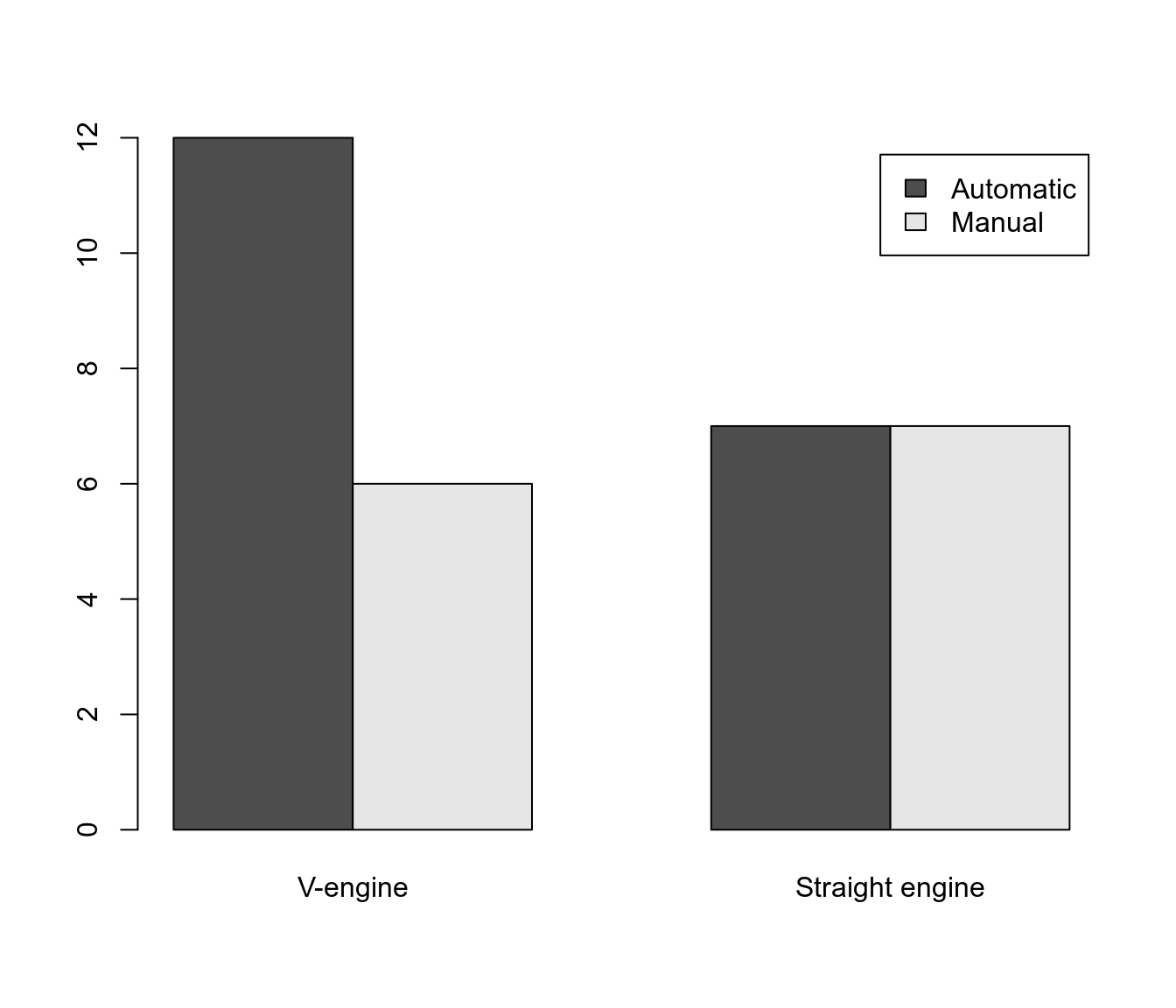
     )

boxplot(mpg ~ am, data = mtcars)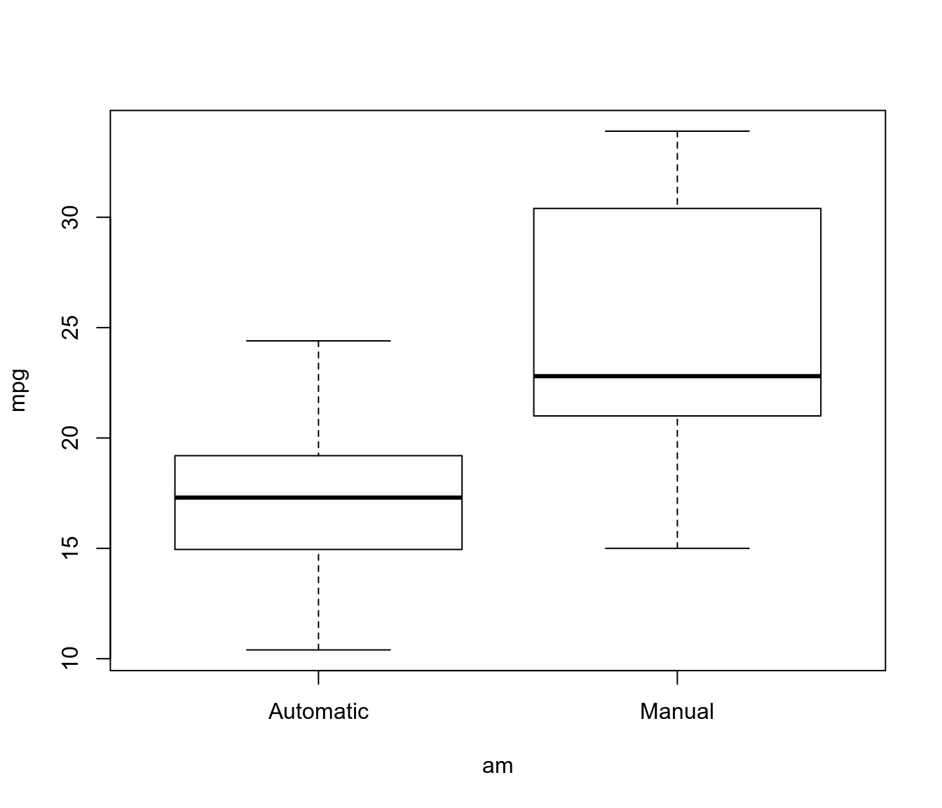

There is a special function for variables labels support - use_labels. By now variables labels support available only for expression which will be evaluated inside data.frame.

# table with dimension names
use_labels(mtcars, table(am, vs))

##             Engine
## Transmission V-engine Straight engine
##    Automatic       12               7
##    Manual           6               7

# linear regression
use_labels(mtcars, lm(mpg ~ wt + hp + qsec)) %>% summary

## 
## Call:
## lm(formula = `Miles/(US) gallon` ~ `Weight (1000 lbs)` + `Gross horsepower` + 
##     `1/4 mile time`)
## 
## Residuals:
## LABEL: Miles/(US) gallon 
## VALUES:
## -3.8591, -1.6418, -0.4636, 1.194, 5.6092
## 
## Coefficients:
##                     Estimate Std. Error t value Pr(>|t|)    
## (Intercept)         27.61053    8.41993   3.279  0.00278 ** 
## `Weight (1000 lbs)` -4.35880    0.75270  -5.791 3.22e-06 ***
## `Gross horsepower`  -0.01782    0.01498  -1.190  0.24418    
## `1/4 mile time`      0.51083    0.43922   1.163  0.25463    
## ---
## Signif. codes:  0 '***' 0.001 '**' 0.01 '*' 0.05 '.' 0.1 ' ' 1
## 
## Residual standard error: 2.578 on 28 degrees of freedom
## Multiple R-squared:  0.8348, Adjusted R-squared:  0.8171 
## F-statistic: 47.15 on 3 and 28 DF,  p-value: 4.506e-11

And, finally, ggplot2 graphics with variables and value labels:

library(ggplot2, warn.conflicts = FALSE)

use_labels(mtcars, {
    # '..data' is shortcut for all 'mtcars' data.frame inside expression 
    ggplot(..data) +
        geom_point(aes(y = mpg, x = wt, color = qsec)) +
        facet_grid(am ~ vs)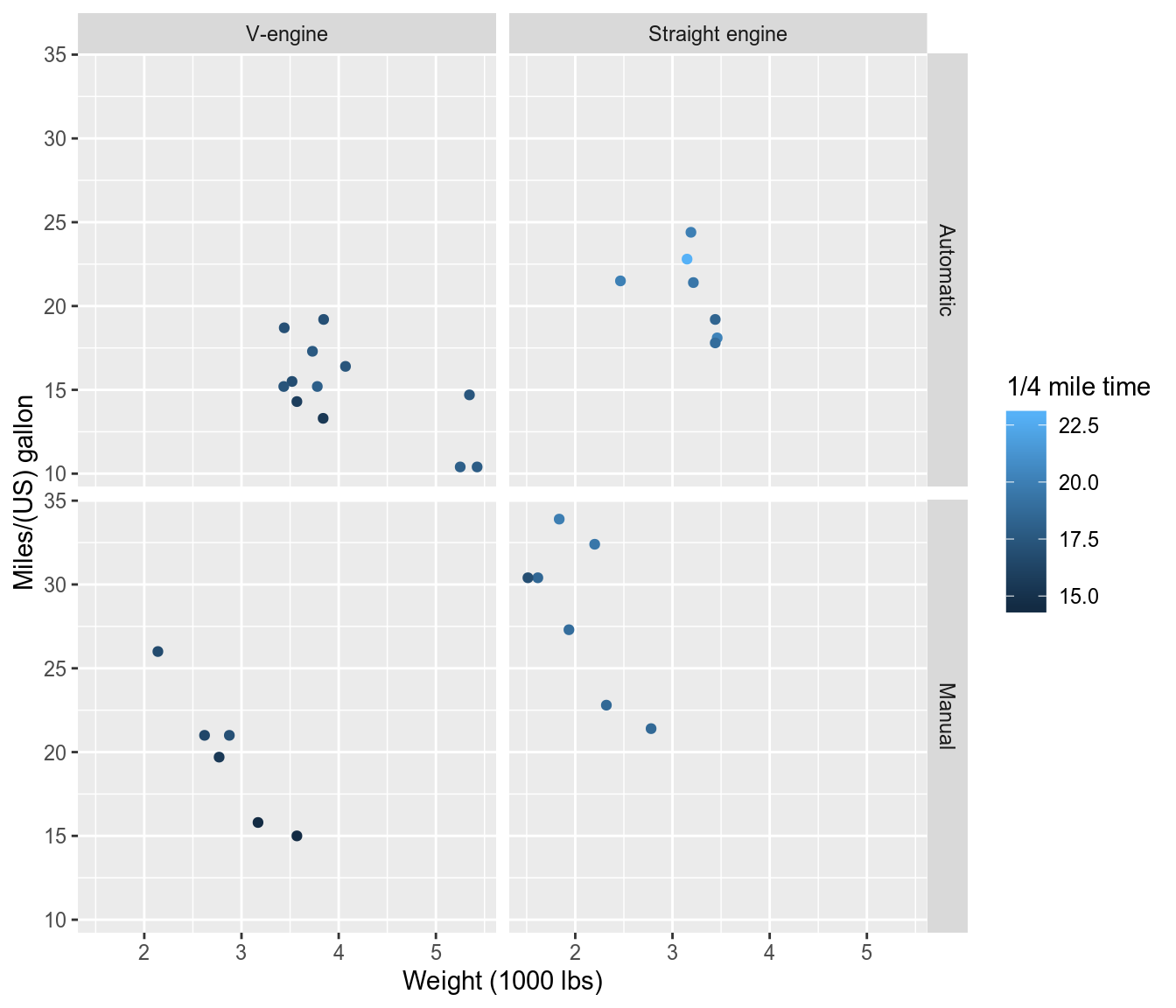
})

Extreme value labels support

We have an option for extreme values lables support: expss_enable_value_labels_support_extreme(). With this option factor/as.factor will take into account empty levels. However, unique will give weird result for labelled variables: labels without values will be added to unique values. That’s why it is recommended to turn off this option immediately after usage. See examples.

We have label ‘Hard to say’ for which there are no values in nps:

nps = c(-1, 0, 1, 1, 0, 1, 1, -1)
var_lab(nps) = "Net promoter score"
val_lab(nps) = num_lab("
            -1 Detractors
             0 Neutralists    
             1 Promoters
             99 Hard to say
")

Here we disable labels support and get results without labels:

expss_disable_value_labels_support()
table(nps) # there is no labels in the result

## nps
## -1  0  1 
##  2  2  4

unique(nps)

## [1] -1  0  1

Results with default value labels support - three labels are here but “Hard to say” is absent.

expss_enable_value_labels_support()
# table with labels but there are no label "Hard to say"
table(nps)

## nps
##  Detractors Neutralists   Promoters 
##           2           2           4

unique(nps)

## LABEL: Net promoter score 
## VALUES:
## -1, 0, 1
## VALUE LABELS:               
##  -1 Detractors 
##   0 Neutralists
##   1 Promoters  
##  99 Hard to say

And now extreme value labels support - we see “Hard to say” with zero counts. Note the weird unique result.

expss_enable_value_labels_support_extreme()
# now we see "Hard to say" with zero counts
table(nps)

## nps
##  Detractors Neutralists   Promoters Hard to say 
##           2           2           4           0

# weird 'unique'! There is a value 99 which is absent in 'nps'
unique(nps)

## LABEL: Net promoter score 
## VALUES:
## -1, 0, 1, 99
## VALUE LABELS:               
##  -1 Detractors 
##   0 Neutralists
##   1 Promoters  
##  99 Hard to say

Return immediately to defaults to avoid issues:

expss_enable_value_labels_support()

Labels are preserved during common operations on the data

There are special methods for subsetting and concatenating labelled variables. These methods preserve labels during common operations. We don’t need to restore labels on subsetted or sorted data.frame.

mtcars with labels:

str(mtcars)

## 'data.frame':    32 obs. of  11 variables:
##  $ mpg :Class 'labelled' num  21 21 22.8 21.4 18.7 18.1 14.3 24.4 22.8 19.2 ...
##    .. .. LABEL: Miles/(US) gallon 
##  $ cyl :Class 'labelled' num  6 6 4 6 8 6 8 4 4 6 ...
##    .. .. LABEL: Number of cylinders 
##  $ disp:Class 'labelled' num  160 160 108 258 360 ...
##    .. .. LABEL: Displacement (cu.in.) 
##  $ hp  :Class 'labelled' num  110 110 93 110 175 105 245 62 95 123 ...
##    .. .. LABEL: Gross horsepower 
##  $ drat:Class 'labelled' num  3.9 3.9 3.85 3.08 3.15 2.76 3.21 3.69 3.92 3.92 ...
##    .. .. LABEL: Rear axle ratio 
##  $ wt  :Class 'labelled' num  2.62 2.88 2.32 3.21 3.44 ...
##    .. .. LABEL: Weight (1000 lbs) 
##  $ qsec:Class 'labelled' num  16.5 17 18.6 19.4 17 ...
##    .. .. LABEL: 1/4 mile time 
##  $ vs  :Class 'labelled' num  0 0 1 1 0 1 0 1 1 1 ...
##    .. .. LABEL: Engine 
##    .. .. VALUE LABELS [1:2]: 0=V-engine, 1=Straight engine 
##  $ am  :Class 'labelled' num  1 1 1 0 0 0 0 0 0 0 ...
##    .. .. LABEL: Transmission 
##    .. .. VALUE LABELS [1:2]: 0=Automatic, 1=Manual 
##  $ gear:Class 'labelled' num  4 4 4 3 3 3 3 4 4 4 ...
##    .. .. LABEL: Number of forward gears 
##  $ carb:Class 'labelled' num  4 4 1 1 2 1 4 2 2 4 ...
##    .. .. LABEL: Number of carburetors

Make subset of the data.frame:

mtcars_subset = mtcars[1:10, ]

Labels are here, nothing is lost:

str(mtcars_subset)

## 'data.frame':    10 obs. of  11 variables:
##  $ mpg :Class 'labelled' num  21 21 22.8 21.4 18.7 18.1 14.3 24.4 22.8 19.2
##    .. .. LABEL: Miles/(US) gallon 
##  $ cyl :Class 'labelled' num  6 6 4 6 8 6 8 4 4 6
##    .. .. LABEL: Number of cylinders 
##  $ disp:Class 'labelled' num  160 160 108 258 360 ...
##    .. .. LABEL: Displacement (cu.in.) 
##  $ hp  :Class 'labelled' num  110 110 93 110 175 105 245 62 95 123
##    .. .. LABEL: Gross horsepower 
##  $ drat:Class 'labelled' num  3.9 3.9 3.85 3.08 3.15 2.76 3.21 3.69 3.92 3.92
##    .. .. LABEL: Rear axle ratio 
##  $ wt  :Class 'labelled' num  2.62 2.88 2.32 3.21 3.44 ...
##    .. .. LABEL: Weight (1000 lbs) 
##  $ qsec:Class 'labelled' num  16.5 17 18.6 19.4 17 ...
##    .. .. LABEL: 1/4 mile time 
##  $ vs  :Class 'labelled' num  0 0 1 1 0 1 0 1 1 1
##    .. .. LABEL: Engine 
##    .. .. VALUE LABELS [1:2]: 0=V-engine, 1=Straight engine 
##  $ am  :Class 'labelled' num  1 1 1 0 0 0 0 0 0 0
##    .. .. LABEL: Transmission 
##    .. .. VALUE LABELS [1:2]: 0=Automatic, 1=Manual 
##  $ gear:Class 'labelled' num  4 4 4 3 3 3 3 4 4 4
##    .. .. LABEL: Number of forward gears 
##  $ carb:Class 'labelled' num  4 4 1 1 2 1 4 2 2 4
##    .. .. LABEL: Number of carburetors

Interaction with ‘haven’

To use expss with haven you need to load expss strictly after haven (or other package with implemented ‘labelled’ class) to avoid conflicts. And it is better to use read_spss with explict package specification: haven::read_spss. See example below. havenpackage doesn’t set ‘labelled’ class for variables which have variable label but don’t have value labels. It leads to labels losing during subsetting and other operations. We have a special function to fix this: add_labelled_class. Apply it to dataset loaded by haven.

# we need to load packages strictly in this order to avoid conflicts
library(haven)
library(expss)
spss_data = haven::read_spss("spss_file.sav")
# add missing 'labelled' class
spss_data = add_labelled_class(spss_data)

Export to Microsoft Excel

To export expss tables to *.xlsx you need to install excellent openxlsx package. To install it just type in the console install.packages("openxlsx"). On Windows system you may need also install RTools. It can be downloaded from CRAN: RTools.

First we apply labels on the mtcars dataset and build simple table with caption.

library(expss)
library(openxlsx)
data(mtcars)
mtcars = apply_labels(mtcars,
                      mpg = "Miles/(US) gallon",
                      cyl = "Number of cylinders",
                      disp = "Displacement (cu.in.)",
                      hp = "Gross horsepower",
                      drat = "Rear axle ratio",
                      wt = "Weight (lb/1000)",
                      qsec = "1/4 mile time",
                      vs = "Engine",
                      vs = c("V-engine" = 0,
                             "Straight engine" = 1),
                      am = "Transmission",
                      am = c("Automatic" = 0,
                             "Manual"=1),
                      gear = "Number of forward gears",
                      carb = "Number of carburetors"
)

mtcars_table = mtcars %>% 
    calc_cro_cpct(
        cell_vars = list(cyl, gear),
        col_vars = list(total(), am, vs)
    ) %>% 
    set_caption("Table 1")

mtcars_table

	#Total	Transmission		Engine
Table 1
		Automatic	Manual	V-engine	Straight engine
Number of cylinders
4	34.4	15.8	61.5	5.6	71.4
6	21.9	21.1	23.1	16.7	28.6
8	43.8	63.2	15.4	77.8
#Total cases	32	19	13	18	14
Number of forward gears
3	46.9	78.9		66.7	21.4
4	37.5	21.1	61.5	11.1	71.4
5	15.6		38.5	22.2	7.1
#Total cases	32	19	13	18	14

Then we create workbook and add worksheet to it.

wb = createWorkbook()
sh = addWorksheet(wb, "Tables")

Export - we should specify workbook and worksheet.

xl_write(mtcars_table, wb, sh)

And, finally, we save workbook with table to the xlsx file.

saveWorkbook(wb, "table1.xlsx", overwrite = TRUE)

Screenshot of the exported table: table1.xlsx

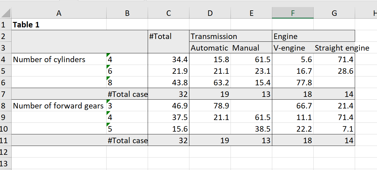
Automation of the report generation

First of all, we create banner which we will use for all our tables.

banner = calc(mtcars, list(total(), am, vs))

Then we generate list with all tables. If variables have small number of discrete values we create column percent table. In other cases we calculate table with means. For both types of tables we mark significant differencies between groups.

list_of_tables = lapply(mtcars, function(variable) {
    if(length(unique(variable))<7){
        cro_cpct(variable, banner) %>% significance_cpct()
    } else {
        # if number of unique values greater than seven we calculate mean
        cro_mean_sd_n(variable, banner) %>% significance_means()
        
    }
    
})

Create workbook:

wb = createWorkbook()
sh = addWorksheet(wb, "Tables")

Here we export our list with tables with additional formatting. We remove ‘#’ sign from totals and mark total column with bold. You can read about formatting options in the manual fro xl_write (?xl_write in the console).

xl_write(list_of_tables, wb, sh, 
         # remove '#' sign from totals 
         col_symbols_to_remove = "#",
         row_symbols_to_remove = "#",
         # format total column as bold
         other_col_labels_formats = list("#" = createStyle(textDecoration = "bold")),
         other_cols_formats = list("#" = createStyle(textDecoration = "bold")),
         )

Save workbook:

saveWorkbook(wb, "report.xlsx", overwrite = TRUE)

Screenshot of the generated report: report.xlsx

Excel functions translation guide

Let us consider Excel toy table:

	A	B	C
1	2	15	50
2	1	70	80
3	3	30	40
4	2	30	40

Code for creating the same table in R:

library(expss)
w = text_to_columns("
        a  b  c
        2 15 50
        1 70 80
        3 30 40
        2 30 40
")

w is the name of our table.

IF

Excel: IF(B1>60, 1, 0)

R: Here we create new column with name d with results. ifelse function is from base R not from ‘expss’ package but included here for completeness.

w$d = ifelse(w$b>60, 1, 0)

If we need to use multiple transformations it is often convenient to use compute function. Inside compute we can put arbitrary number of the statements:

w = compute(w, {
    d = ifelse(b>60, 1, 0)
    e = 42
    abc_sum = sum_row(a, b, c)
    abc_mean = mean_row(a, b, c)
})

COUNTIF

Count 1’s in the entire dataset.

Excel: COUNTIF(A1:C4, 1)

count_if(1, w)

calculate(w, count_if(1, a, b, c))

Count values greater than 1 in each row of the dataset.

Excel: COUNTIF(A1:C1, ">1")

w$d = count_row_if(gt(1), w)

w = compute(w, {
    d = count_row_if(gt(1), a, b, c) 
})

Count values less than or equal to 1 in column A of the dataset.

Excel: COUNTIF(A1:A4, "<=1")

count_col_if(le(1), w$a)

Table of criteria:

Excel	R
<1	lt(1)
<=1	le(1)
<>1	ne(1)
=1	eq(1)
>=1	ge(1)
>1	gt(1)

SUM/AVERAGE

Sum all values in the dataset.

Excel: SUM(A1:C4)

sum(w, na.rm = TRUE)

Calculate average of each row of the dataset.

Excel: AVERAGE(A1:C1)

w$d = mean_row(w)

w = compute(w, {
    d = mean_row(a, b, c) 
})

Sum values of column A of the dataset.

Excel: SUM(A1:A4)

sum_col(w$a)

SUMIF/AVERAGEIF

Sum values greater than 40 in the entire dataset.

Excel: SUMIF(A1:C4, ">40")

sum_if(gt(40), w)

calculate(w, sum_if(gt(40), a, b, c))

Sum values less than 40 in the each row of the dataset.

Excel: SUMIF(A1:C1, "<40")

w$d = sum_row_if(lt(40), w)

w = compute(w, {
    d = sum_row_if(lt(40), a, b, c) 
})

Calculate average of B column with column A values less than 3.

Excel: AVERAGEIF(A1:A4, "<3", B1:B4)

mean_col_if(lt(3), w$a, data = w$b)

or, if we want calculate means for both b and c columns:

calculate(w, mean_col_if(lt(3), a, data = sheet(b, c)))

VLOOKUP

Our dictionary for lookup:

	X	Y
1	1	apples
2	2	oranges
3	3	peaches

Code for creating the same dictionary in R:

dict = text_to_columns("
    x  y
    1  apples
    2  oranges
    3  peaches
")

Excel: VLOOKUP(A1, $X$1:$Y$3, 2, FALSE)

w$d = vlookup(w$a, dict, 2)

or, we can use column names:

w$d = vlookup(w$a, dict, "y")

SPSS functions translation guide

COMPUTE

SPSS:

COMPUTE d = 1.

w$d = 1

or, in the specific data.frame

w = compute(w, {
    d = 1
})

There can be arbitrary number of statements inside compute.

IF

SPSS:

IF(a = 3) d = 2.

w = compute(w, {
    d = ifelse(a == 3, 2, NA)
})

or,

w = compute(w, {
    d = ifs(a == 3 ~ 2)
})

DO IF

SPSS:

DO IF (a>1).
    COMPUTE d = 4.
END IF.

w = do_if(w, a>1, {
    d = 4
})

There can be arbitrary number of statements inside do_if.

COUNT

SPSS:

COUNT cnt = a1 TO a5 (LO THRU HI).

cnt = count_row_if(lo %thru% hi, a1 %to% a5)

SPSS:

COUNT cnt = a1 TO a5 (SYSMIS).

cnt = count_row_if(NA, a1 %to% a5)

SPSS:

COUNT cnt = a1 TO a5 (1 THRU 5).

cnt = count_row_if(1 %thru% 5, a1 %to% a5)

SPSS:

COUNT cnt = a1 TO a5 (1 THRU HI).

cnt = count_row_if(1 %thru% hi, a1 %to% a5)

or,

cnt = count_row_if(ge(1), a1 %to% a5)

SPSS:

COUNT cnt = a1 TO a5 (LO THRU 1).

cnt = count_row_if(lo %thru% 1, a1 %to% a5)

or,

cnt = count_row_if (le(1), a1 %to% a5)

SPSS:

COUNT cnt = a1 TO a5 (1 THRU 5, 99).

cnt = count_row_if(1 %thru% 5 | 99, a1 %to% a5)

SPSS:

COUNT cnt = a1 TO a5(1,2,3,4,5, SYSMIS).

cnt = count_row_if(c(1:5, NA), a1 %to% a5)

count_row_if can be used inside compute.

RECODE

SPSS:

RECODE V1 (0=1) (1=0) (2, 3=-1) (9=9) (ELSE=SYSMIS)

recode(v1) = c(0 ~ 1, 1 ~ 0, 2:3 ~ -1, 9 ~ 9, other ~ NA)

SPSS:

RECODE QVAR(1 THRU 5=1)(6 THRU 10=2)(11 THRU HI=3)(ELSE=0).

recode(qvar) = c(1 %thru% 5 ~ 1, 6 %thru% 10 ~ 2, 11 %thru% hi ~ 3, other ~ 0)

SPSS:

RECODE STRNGVAR ('A', 'B', 'C'='A')('D', 'E', 'F'='B')(ELSE=' ').

recode(strngvar) = c(c('A', 'B', 'C') ~ 'A', c('D', 'E', 'F') ~ 'B', other ~ ' ')

SPSS:

RECODE AGE (MISSING=9) (18 THRU HI=1) (0 THRU 18=0) INTO VOTER.

voter = recode(age, NA ~ 9, 18 %thru% hi ~ 1, 0 %thru% 18 ~ 0)
# or
recode(age, NA ~ 9, 18 %thru% hi ~ 1, 0 %thru% 18 ~ 0) %into% voter

recode can be used inside compute.

VARIABLE LABELS

SPSS:

VARIABLE LABELS a "Fruits"
                b "Cost"
                c "Price".

w = apply_labels(w,
                 a = "Fruits",
                 b = "Cost",
                 c = "Price"
)

VALUE LABELS

SPSS:

VALUE LABELS a
    1 "apples"
    2 "oranges"
    3 "peaches".

w = apply_labels(w, 
                 a = num_lab("
                        1 apples
                        2 oranges
                        3 peaches 
                    ")
)

or,

val_lab(w$a) = num_lab("
    1 apples
    2 oranges
    3 peaches 
")

Tables

fre(w$a) # Frequency of fruits

Fruits	Count	Valid percent	Percent	Responses, %	Cumulative responses, %
apples	1	25	25	25	25
oranges	2	50	50	50	75
peaches	1	25	25	25	100
#Total	4	100	100	100
<NA>	0		0

cro_cpct(w$b, w$a) # Column percent of cost by fruits

	Fruits
	apples	oranges	peaches
Cost
15		50
30		50	100
70	100
#Total cases	1	2	1

cro_mean(sheet(w$b, w$c), w$a) # Mean cost and price by fruits

	Fruits
	apples	oranges	peaches
Cost	70	22.5	30
Price	80	45.0	40

저작자표시 변경금지

'R' 카테고리의 다른 글

moonBook 패키지를 이용한 도넛 원그래프 작성하기 (0)	2018.12.27
plotly 패키지를 이용한 원그래프 그리기 (0)	2018.12.27
특정한 데이터 유형을 갖는 열을 추출하기 (0)	2018.12.26
type() 함수와 mode() 함수의 차이에 대한 이해 (0)	2018.12.16
Jupyter Notebook에 R연동하기 (0)	2018.12.11

ABOUT ME

buillee buillee

expss: Tables with Labels in R

2018-11-12

Introduction

Links

Installation

Cross-tablulation examples

Example of data processing with multiple-response variables

Labels support for base R

Getting and setting variable and value labels

Labels with base R and ggplot2 functions

Extreme value labels support

Labels are preserved during common operations on the data

Interaction with ‘haven’

Export to Microsoft Excel

Automation of the report generation

Excel functions translation guide

IF

COUNTIF

SUM/AVERAGE

SUMIF/AVERAGEIF

VLOOKUP

SPSS functions translation guide

COMPUTE

IF

DO IF

COUNT

RECODE

VARIABLE LABELS

VALUE LABELS

Tables

'R' 카테고리의 다른 글

티스토리툴바

ABOUT ME

expss: Tables with Labels in R

2018-11-12

Introduction

Links

Installation

Cross-tablulation examples

Example of data processing with multiple-response variables

Labels support for base R

Getting and setting variable and value labels

Labels with base R and ggplot2 functions

Extreme value labels support

Labels are preserved during common operations on the data

Interaction with ‘haven’

Export to Microsoft Excel

Automation of the report generation

Excel functions translation guide

IF

COUNTIF

SUM/AVERAGE

SUMIF/AVERAGEIF

VLOOKUP

SPSS functions translation guide

COMPUTE

IF

DO IF

COUNT

RECODE

VARIABLE LABELS

VALUE LABELS

Tables

'R' 카테고리의 다른 글

관련글 관련글 더보기

티스토리툴바